
This article is a joint compilation: Blake, Gao Fei
Lei Fengnet (search "Lei Feng Net" public concern) Note: Prof. Yoshua Bengio is one of the machine learning gods, especially in the field of deep learning, he is also the author of "Learning Deep Architectures for AI" in the artificial intelligence field. . Yoshua Bengio, along with Professor Geoff Hinton and Professor Yann LeCun, created the deep learning revival that began in 2006. His research work focuses on advanced machine learning and is dedicated to solving artificial intelligence problems. He is currently one of the few remaining deep learning professors still fully involved in academia (University of Montreal). This article is the first part of his content in the classic forward-looking speech in 2009, “In-depth Architecture of Artificial Intelligence Learningâ€. .
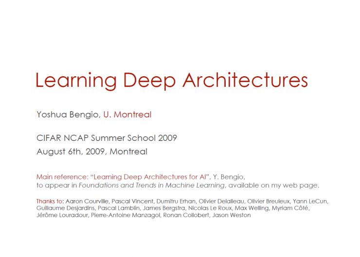
Artificial intelligence learning depth architecture
Yoshua Bengio University of Montreal
Main content: "Artificial intelligence learning depth architecture" Â 
Depth architecture works well
Defeat a shallow neural network in visual and natural language processing tasks
Failed support vector machines (SVMs) in pixel-level vision tasks (at the same time able to handle data sizes that SVMs cannot handle in natural language processing problems)
Realizes the best performance in the field of natural language processing
Defeated deep neural networks in an unsupervised state
Learned visual characteristics (similar to V1 and V2 neurons)
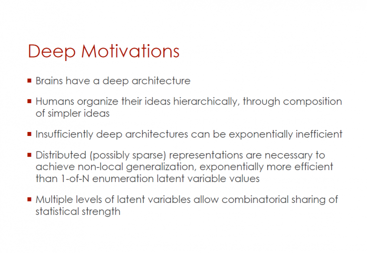
Depth architecture motivation
The brain has a deep architecture
Human beings think hierarchically (by constructing some simple concepts)
Insufficient depth of architecture also reduces its efficiency
Distributed characterization (possibly sparse) is necessary for non-localized generalization, much more efficient than 1-N enumeration of latent variable values
Multilevel latent variables allow sharing combinations of statistical intensities
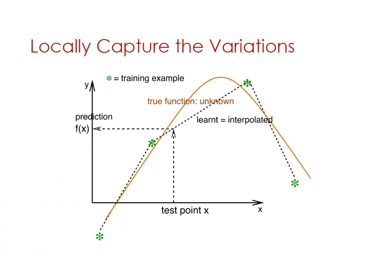
Locally captured variables
The vertical axis is the prediction f(x), and the horizontal axis is the test point x

With less simple case of variable
Purple curve represents true unknown operation
The blue curve represents what has been learned: where prediction = f(x)
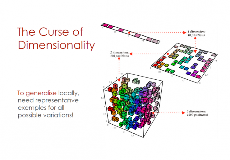
The curse of the dimension
1 dimensional time - 10 positions
2D time - 100 positions
3D time - 1000 positions
To achieve a local overview, a sample representation of all possible variables is required.

Limitations of Local Generalization: Theoretical Results (Bengio & Delalleau 2007)
Theory: A Gaussian kernel machine needs at least k samples to learn an operation (2k zero crossings on some lines)
Theory: For Gaussian kernel machines, dimensional training of multiple functions requires cross-dimensional samples
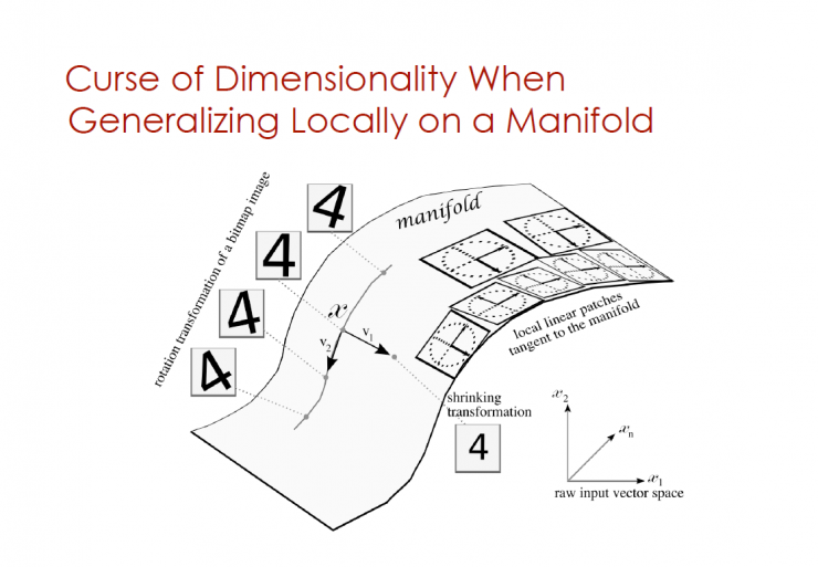
Dimensional Dimensionality When Generalizing Locally on a Manifold
Rotation transformation of a bitmap image
Local linear patches tangent to the manifold
Shrinking transformation
Raw input vector space
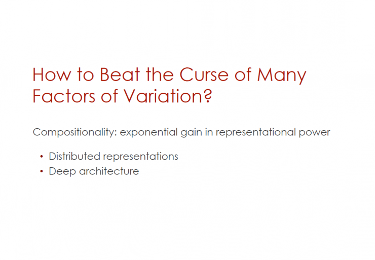
How to defeat the curse of many factors in the variable?
Combinatorial: exponential gain in characterization
Distribution representations (Distributed representations)
Deep architecture
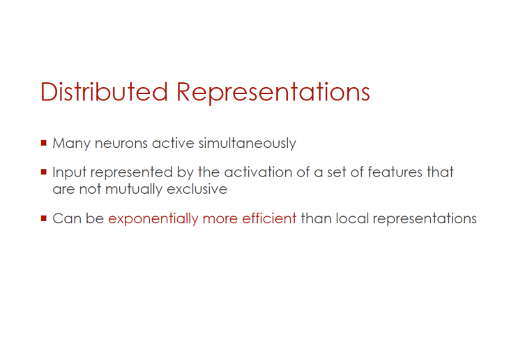
Distribution representations (Distributed representations)
Many neurons are simultaneously active
Entering activities that represent a series of features that are not independent of each other
More effective than local characterization (exponential)

Local VS distribution
Local partitioning: Partitioning by learning to prototype
Distributed Partition: Child Partition 1, Child Partition 2, Child Partition 3
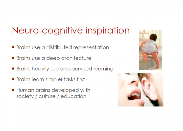
Cognitive Neuroscience Inspiration
The brain uses a distributed representation
The brain is also a deep architecture
Heavy brain use of unsupervised learning
The brain tends to learn simpler tasks
The human brain develops through social/cultural/educational development
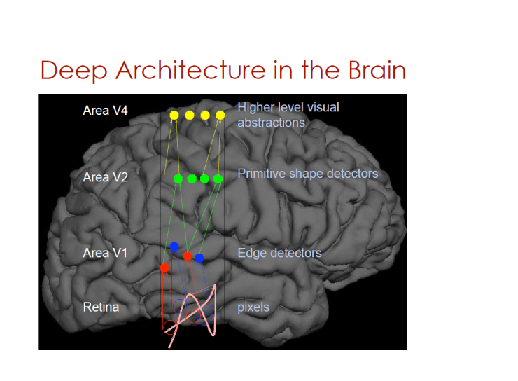
Deep architecture in the brain
V4 area - higher level visual abstraction
V3 area - primary shape detector
V2 area - edge detector
Retina - Pixel
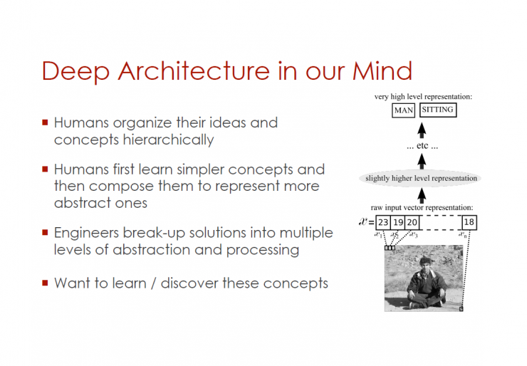
Deep structure in our mind (mind)
Humans organize their ideas and concepts hierarchically
Humans first learn some simpler concepts and then combine them to represent more complex abstract concepts.
Engineers divide the solution into multiple levels of abstraction and processing
Want to learn/discover these concepts
Example:
From the picture (the man sitting on the ground) - the original input vector representation - the slightly higher order representation - the middle level etc. - quite high level representation (man, sitting)
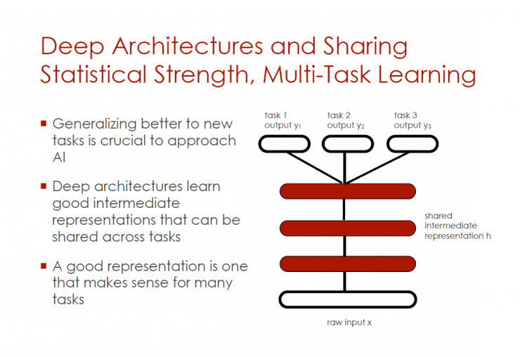
Deep architecture and shared statistical strength and multi-task learning
If you want to be closer to artificial intelligence, it is crucial to better promote new tasks.
Deep architecture can learn good intermediate representations (can be shared between tasks)
A good characterization is meaningful for many tasks
Original input x - shared intermediate representation h - tasks 1, 2, 3 (y1, y2, y3)
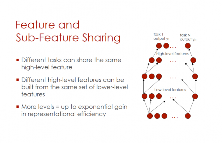
Sharing features and subfeatures
Different tasks can share the same high-level features
Different high-order features can be built from the same low-order feature group
More levels = exponentially increased in characterization
Low-order features - higher-order features - task 1-N (output y1-yN)
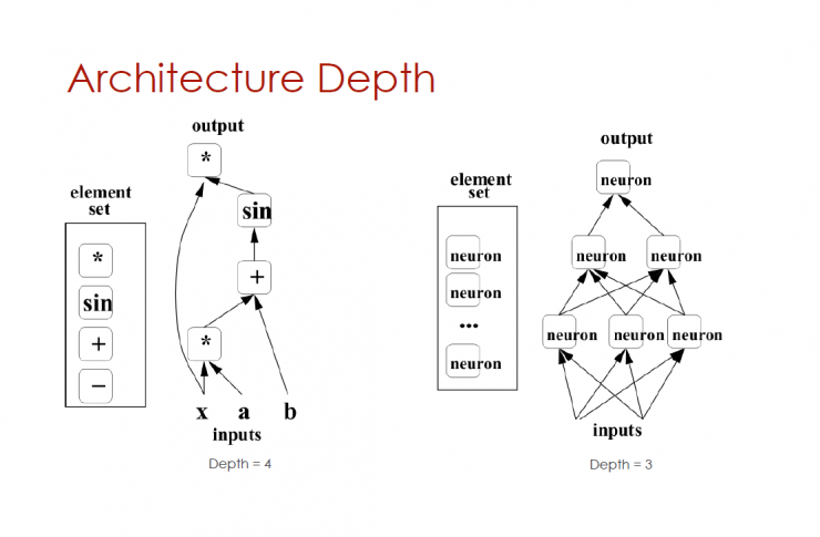
Depth of architecture
Element Set (, sin, +, -) - Input (x, a, b) Output () Depth = 4
Element sets (neurons, neurons, neurons) - depth = 3
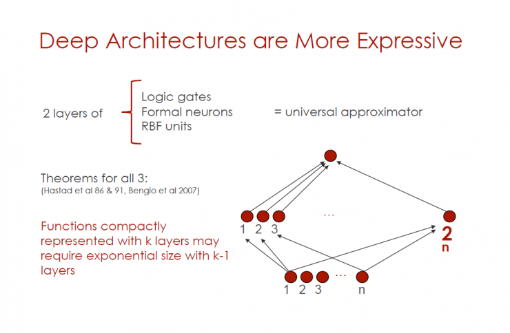
Deeper architecture is more expressive
Layer 2 (logic gate, formal neuron, RBF unit) = Universal Approximator
All three principles (Hastad et al 86 & 91, Bengio et al 2007)
Closely characterized operations using k layers may require k-1 layer exponential levels
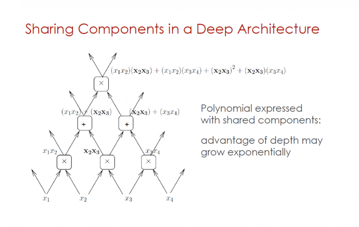
Sharing components in deep architecture
Polynomials with shared components: The advantages of depth may grow exponentially
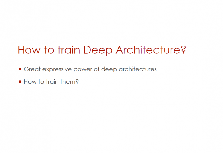
How to train deep architecture?
Deep architecture has powerful characterization capabilities
How to train them?

Breakthrough in depth
Prior to 2006, the training depth architecture was unsuccessful (except for convolutional neural networks)
Hinton, Osindero & Teh « A Fast Learning Algorithm for Deep Belief Nets », Neural Computation, 2006
Bengio, Lamblin, Popovici, Larochelle « Greedy Layer-Wise Training of Deep Networks », NIPS'2006
Ranzato, Poultney, Chopra, LeCun « Efficient Learning of Sparse Representations with an Energy-Based Model », NIPS'2006
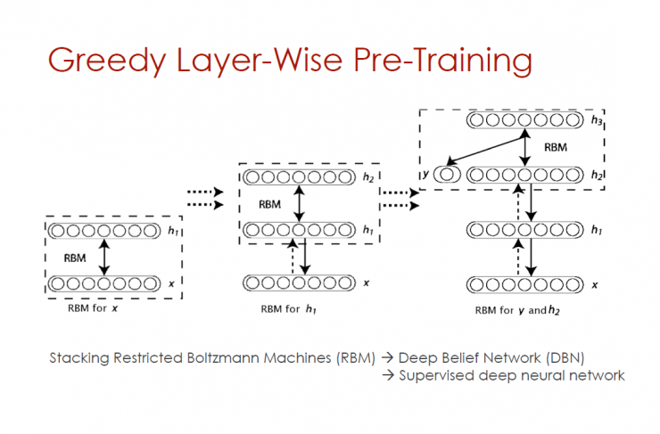
Greedy level-by-layer pre-training
Stack Restricted Boltzmann Machine (RBM) - Deep Belief Network (DBN) - Supervise Deep Neural Networks

Good multilayer neural network
Each output vector
Given the input x output layer prediction parameter distribution of the target variable Y
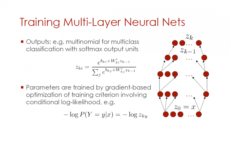
Training multilayer neural networks
Output: Example - Multi-class classification of polynomial and softmax output units
Gradient-optimized training criteria, including conditional logistic training, etc.
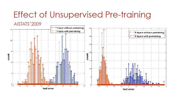
Unsupervised pre-training effect
AISTATS'2009
The horizontal axis represents the test error and the vertical axis represents the count
Blue is pre-trained with no pre-trained orange
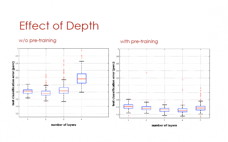
The impact of depth
The horizontal axis is the number of levels, and the vertical axis is the test classification error
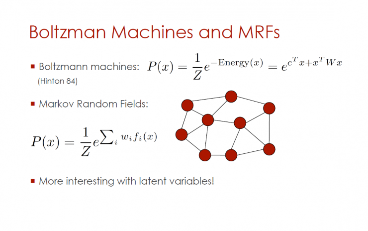
Boltzmann machines and MRFs
Boltzmann machine
Markov Random Field
Hidden variables are more interesting
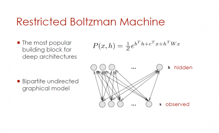
Restricted Boltzmann Machine
The most popular deep architecture components
Bidirectional unsupervised graphics model
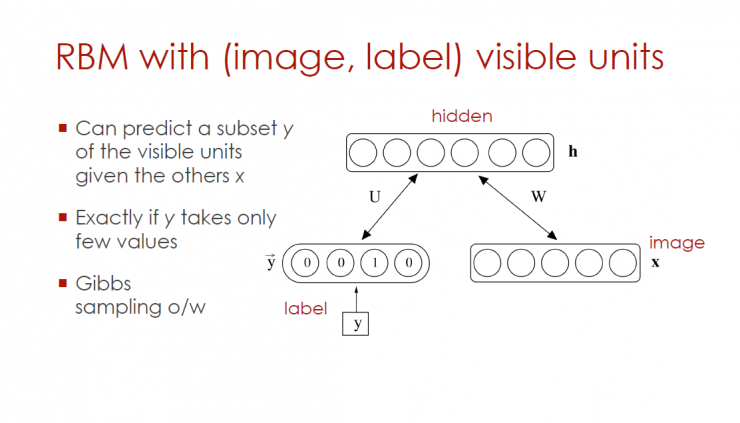
RBM visible unit with (image, mark)
Can predict subset y of visible cells (given other x)
If y gets only a few values
Gibbs sampling
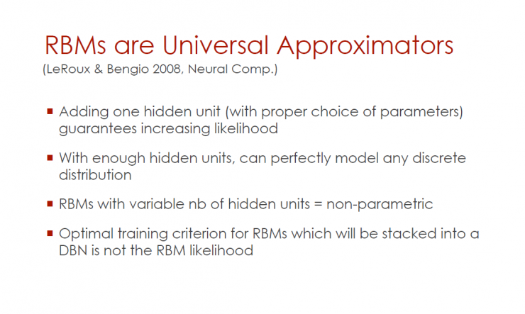
RBMs are universal approximators (LeRoux & Bengio 2008, Neural Comp.)
Adding a hidden unit (with appropriate parameter selection) guarantees increased possibilities
Has enough hidden units to perfectly simulate any discrete distribution
RBMs with nb-level hidden units = non-parametric
Optimal training criterion for RBMs which will be stacked into a DBN is not the RBM likelihood
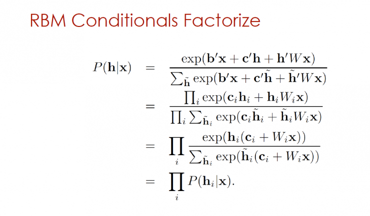
RBM Condition Factorization
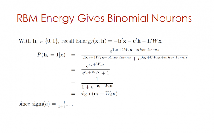
RBM gives binomial neuron energy
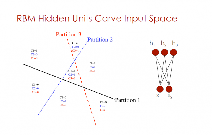
RBM hidden neuron partitioning input controls
Partition 1, Partition 2, Partition 3
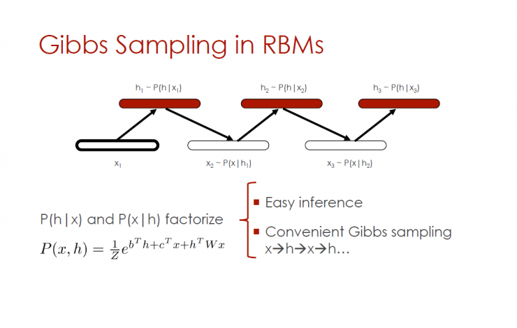
Gibbs sampling in RBMs
P(h|x) and P(x|h) Factorization - Simple Reasoning, Convenient Gibbs Sampling
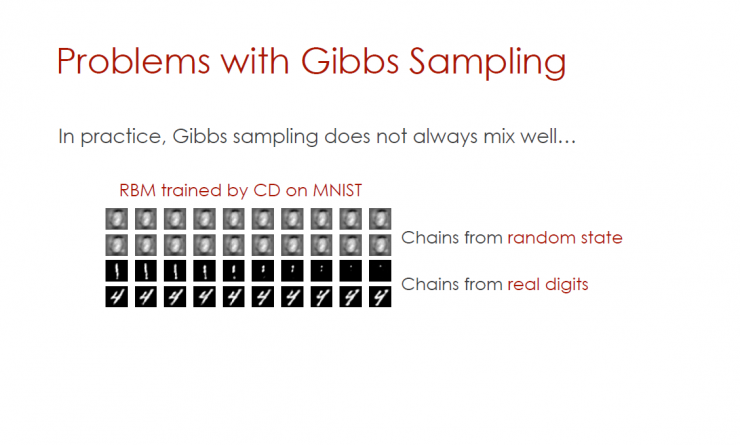
Problems with Gibbs Sampling
In practice, Gibbs sampling is not always a good mix.
Training RBM with CD on MNIST
Random chain
Real digital chain
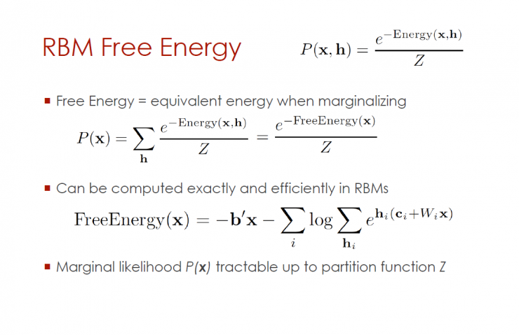
Free energy
Free energy = equivalent energy at marginalization
Accurately and efficiently calculated in RBMs
Marginal likelihood p(x) goes back to the high division function Z
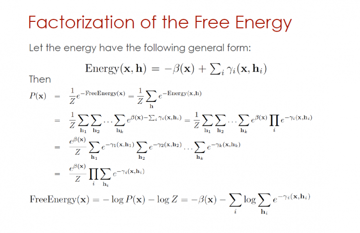
Factorization of free energy
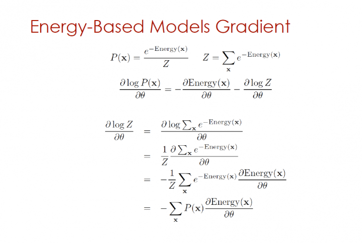
Energy-based model gradient

Boltzmann Machine Gradient
Gradient has two components - positive phase, negative phase
In RBMs, easy to sample or sum in h|x
Different parts: sampling from P(x) using Markov chains

Training RBMs
Contrasting divergence (CD-k) : negative Gibbs chain observation x, run k Gibbs step
Continuous contrast divergence (PCD) : running a negative Gibbs chain in the background when the weight changes slowly
Fast PCD : Two sets of weights, useful for a large number of learning rates only for negative, rapid exploration patterns
Cluster : Deterministic near-chaotic dynamic systems define learning and sampling
Annealing MCMC : Use Higher Temperatures to Avoid Mode
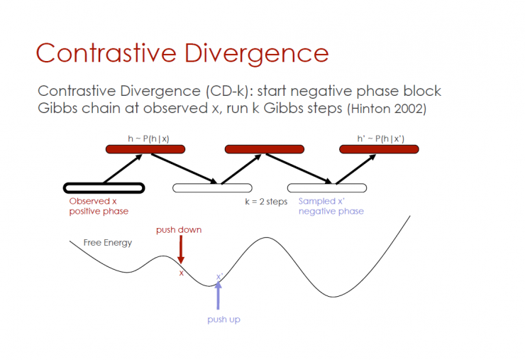
Contrast divergence
Contrasting divergence (CD-k): starting from the negative phase block Gibbs chain observation x, running k Gibbs step (Hinton 2002)
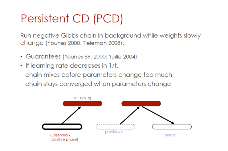
Continuous contrast divergence (PCD)
Run negative Gibbs chains in the background when weights change slowly (Younes 2000, Tieleman 2008):
Guarantee (Younes 89, 2000; Yuille 2004)
If the learning rate is reduced by 1/t
Mix the chain before the parameters change too much
When the parameters change, the chain keeps convergence
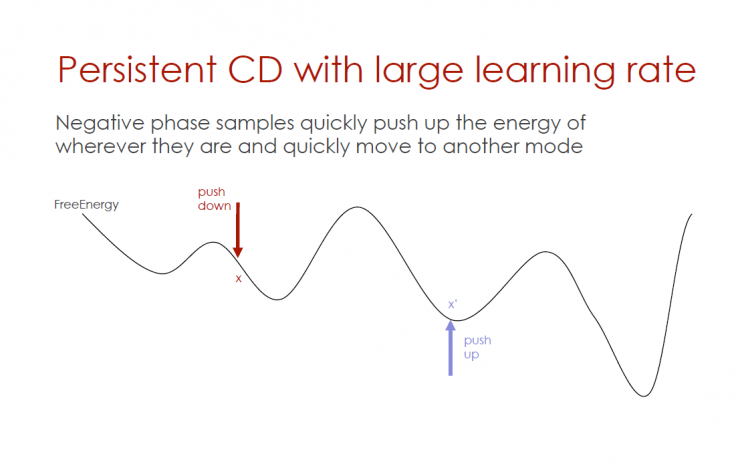
Persistent CD with high learning efficiency
Without considering the location of the energy, the reverse-phase sample quickly pushes up the energy and quickly moves to another mode.
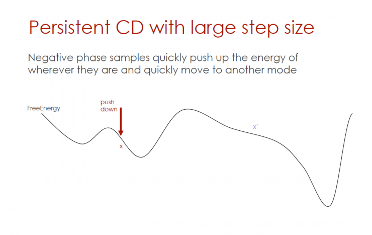
Large stride sustained divergence (persistent CD)
Without considering the location of the energy, the reverse-phase sample quickly pushes up the energy and quickly moves to another mode.

Persistent CD with high learning efficiency
Without considering the location of the energy, the reverse-phase sample quickly pushes up the energy and quickly moves to another mode.

Fast and continuous comparison of divergence and clustering
In the sampling process, the extremely fast clustering effect obtained when the parameters are rapidly changed (high learning efficiency) is utilized.
Fast PCD: Two sets of weight values, one of which corresponds to high learning efficiency, is used only for the reverse phase, and can quickly switch modes.
Clustering (see Max Welling's speech at the ICML, UAI and special lectures): 0 degree MRFs and RBMs to quickly calculate weight values.
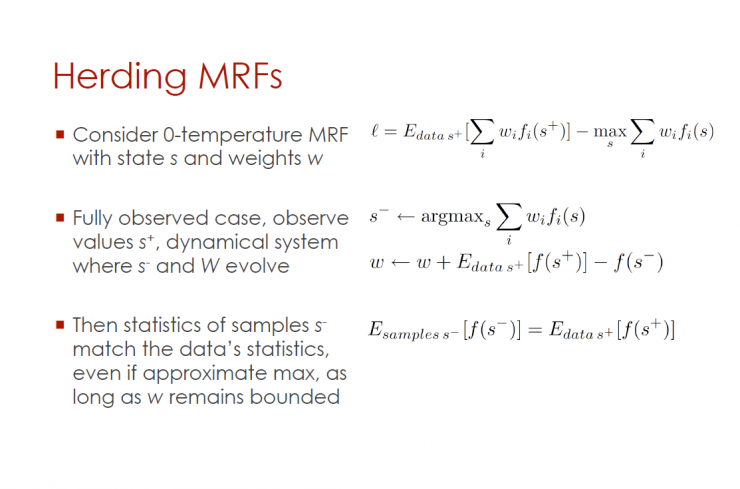
Cluster Markov Random Fields (MRFs)
O degree MRF state S, weight W
A comprehensive observation of the case, the observed results are that there has been a change in the dynamic system and W.
As long as W remains constant, even if the maximum approximation is taken, the statistical results of the sample will still match the statistical results of the data.
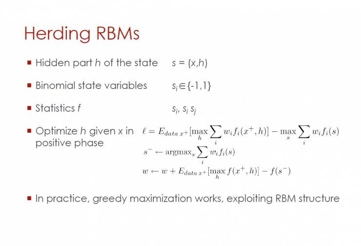
Restricted Boltzmann Machines (RBMs)
The hidden layer of this state s = (x,h)
Binomial State Variables
Statistical value f
In the positive phase, given the input information x, optimize the hidden layer h
In practical operation, using a RBM (restricted Boltzmann machine) structure, the function value can be maximized.
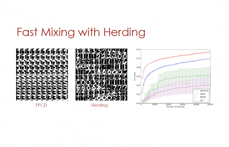
Use clusters for rapid mixing
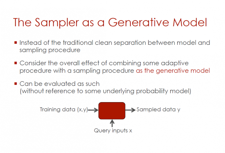
Act as a sampler for the generation model
Cancel the traditional separation between the model and the sampling process
Consider the overall impact of combining adaptive procedures with a sampling program that acts as a generative model
Sampling results can be evaluated through the following steps (without reference to a potential probability model)
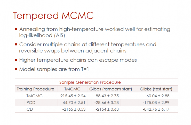
Annealed MCMC (Tempered MCMC)
High temperature annealing helps to estimate the log likelihood
Considering the reversible exchange between multiple chains and adjacent chains under different temperature conditions
Higher temperature chains can be model-free
Model sampling starts from T=1
Summary : This article mainly mentions the related content of deep architecture, neural networks, Boltzmann machines, and why they are applied in the field of artificial intelligence. As Yoshua Bengio's speech in 2009, it is quite forward-looking. In the follow-up section, Yoshua Bengio also mentioned DBN, unsupervised learning and other related concepts and practice process, please continue to pay attention to our next part of the content of the article.
PS: This article was compiled by Lei Fengnet and refused to be reproduced without permission!
Via Yoshua Bengio