The image is represented using one-dimensional coordinates, and while 2D and 3D representations are more complex to visualize, they aren't necessary here. I won’t be using MATLAB, but the concept can still be clearly conveyed.
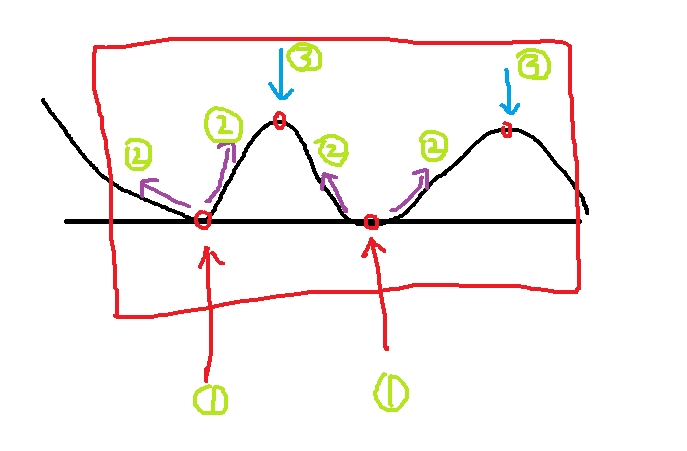
Step 1: Identify the local minimum points in the image. There are several methods to do this—using a kernel or comparing pixel values directly. It’s not too difficult to implement.
Step 2: Begin filling from the lowest point. Water starts to fill the image, which is essentially a gradient-based process. The marked local minima remain dry, while intermediate points get submerged.
Step 3: Locate the local maximum points, which correspond to the three key positions in the figure.
Step 4: Use these local minima and maxima to segment the image.
Classification map
Simulation result graph
Does it feel like this method is efficient and simple? Let's take a look at the next image:
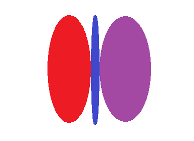
Using the above steps, we first identified three local minima. In the second step, water started to flood, and all three were recorded. Then, two local maxima were found.
Is that what we wanted?
The answer is no. We don’t want the small, insignificant local minimums, as they may just represent noise. We don’t need such fine-grained segmentation.
This shows some flaws. But don’t worry, OpenCV has an improved version of the watershed algorithm that solves this issue.
Analog classification map
Simulation result graph
Improved watershed algorithm in OpenCV:
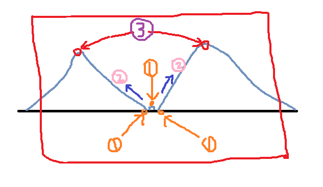
To address the issues mentioned earlier, we considered whether we could mark certain details so that they wouldn't be counted as true local minima.
The OpenCV improvement involves manual marking. You can label specific points, and these labels guide the watershed algorithm. The results are very effective!
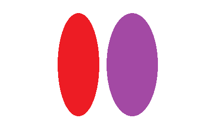
For example, if we mark two triangles on the image, during the first step, we find three local minima. When water floods, all three are submerged. However, if the middle one isn’t marked, it gets submerged (no lifebuoy), while the other two remain, achieving the desired result.
Note: The markings here use different labels. I used the same triangle for simplicity. Since labels are used for classification, different regions should have different labels. This is reflected in the OpenCV code below.
Analog classification map
Simulation result graph
Note: The actual implementation isn’t complete. I believe the principle is sufficient for now. I will study the algorithm in depth when needed. Once you understand the concept, you can adapt it. The interview is over. That’s okay! Hahaha~
OpenCV Implementation:
#include
#include
using namespace cv;
using namespace std;
void waterSegment(InputArray& _src, OutputArray& _dst, int& noOfSegment);
int main(int argc, char** argv) {
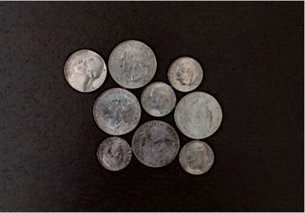
Mat inputImage = imread("coins.jpg");
assert(!inputImage.data);
Mat grayImage, outputImage;
int offSegment;
waterSegment(inputImage, outputImage, offSegment);
waitKey(0);
return 0;
}
void waterSegment(InputArray& _src, OutputArray& _dst, int& noOfSegment)
{
Mat src = _src.getMat();
Mat grayImage;
cvtColor(src, grayImage, CV_BGR2GRAY);
threshold(grayImage, grayImage, 0, 255, THRESH_BINARY | THRESH_OTSU);
Mat kernel = getStructuringElement(MORPH_RECT, Size(9, 9), Point(-1, -1));
morphologyEx(grayImage, grayImage, MORPH_CLOSE, kernel);
distanceTransform(grayImage, grayImage, DIST_L2, DIST_MASK_3, 5);
normalize(grayImage, grayImage, 0, 1, NORM_MINMAX);
grayImage.convertTo(grayImage, CV_8UC1);
threshold(grayImage, grayImage, 0, 255, THRESH_BINARY | THRESH_OTSU);
morphologyEx(grayImage, grayImage, MORPH_CLOSE, kernel);
vector
vector
Mat showImage = Mat::zeros(grayImage.size(), CV_32SC1);
findContours(grayImage, contours, hierarchy, RETR_TREE, CHAIN_APPROX_SIMPLE, Point(-1, -1));
for (size_t i = 0; i < contours.size(); i++)
{
// Here, static_cast
drawContours(showImage, contours, static_cast
}
Mat k = getStructuringElement(MORPH_RECT, Size(3, 3), Point(-1, -1));
morphologyEx(src, src, MORPH_ERODE, k);
watershed(src, showImage);
// Assign random colors
vector
for (size_t i = 0; i < contours.size(); i++) {
int r = theRNG().uniform(0, 255);
int g = theRNG().uniform(0, 255);
int b = theRNG().uniform(0, 255);
Colors.push_back(Vec3b((uchar)b, (uchar)g, (uchar)r));
}
// Display
Mat dst = Mat::zeros(showImage.size(), CV_8UC3);
int index = 0;
for (int row = 0; row < showImage.rows; row++) {
for (int col = 0; col < showImage.cols; col++) {
index = showImage.at
if (index > 0 && index <= contours.size()) {
dst.at
} else if (index == -1) {
dst.at
} else {
dst.at
}
}
}
}
Watershed merge code:
void segMerge(Mat& image, Mat& segments, int& numSeg)
{
vector
int newNumSeg = numSeg;
// Initialize the size of the vector
for (size_t i = 0; i < newNumSeg; i++) {
Mat sample;
Samples.push_back(sample);
}
for (size_t i = 0; i < segments.rows; i++) {
for (size_t j = 0; j < segments.cols; j++) {
int index = segments.at
if (index >= 0 && index <= newNumSeg) {
if (!samples[index].data) {
samples[index] = image(Rect(j, i, 1, 1));
} else {
vconcat(samples[index], image(Rect(j, i, 2, 1)), samples[index]);
}
}
}
}
vector
Mat hsv_base;
int h_bins = 35;
int s_bins = 30;
int histSize[2] = { h_bins, s_bins };
float h_range[2] = { 0, 256 };
float s_range[2] = { 0, 180 };
const float* range[2] = { h_range, s_range };
int channels[2] = { 0, 1 };
Mat hist_base;
for (size_t i = 1; i < numSeg; i++) {
if (samples[i].dims > 0) {
cvtColor(samples[i], hsv_base, CV_BGR2HSV);
calcHist(&hsv_base, 1, channels, Mat(), hist_base, 2, histSize, range);
normalize(hist_base, hist_base, 0, 1, NORM_MINMAX);
Hist_bases.push_back(hist_base);
} else {
Hist_bases.push_back(Mat());
}
}
double similarity = 0;
vector
for (size_t i = 0; i < hist_bases.size(); i++) {
for (size_t j = i + 1; j < hist_bases.size(); j++) {
if (!merged[j]) {
if (hist_bases[i].dims > 0 && hist_bases[j].dims > 0) {
similarity = compareHist(hist_bases[i], hist_bases[j], HISTCMP_BHATTACHARYYA);
if (similarity > 0.8) {
merged[j] = true;
if (i != j) {
newNumSeg--;
for (size_t p = 0; p < segments.rows; p++) {
for (size_t k = 0; k < segments.cols; k++) {
int index = segments.at
if (index == j) segments.at
}
}
}
}
}
}
}
}
numSeg = newNumSeg;
}
Huawei Touch Screen Price,Mobile Phone Touch Panel,Mobile Phone LCD,Mobile Touch Screen Manufacturers
Dongguan Jili Electronic Technology Co., Ltd. , https://www.jlglassoca.com